Magic Formula (Part IV)
Quantopian's Algorithm API is a robust and efficient tool to backtest the Magic Formula Strategy. The algorithm
runs the pipeline to screen for stocks during each period, creating a factor ranking that can be
used to determine which securities to buy or sell during each rebalance.
Running a 15 Year backtest from 2003 to 2018, we find a small positive Sharpe from our two factor model, with the strategy generating annual returns of 9.88% on a Sharpe of 0.55.
Get the Book: The Little Book that Beats the Market
Parts:
One , Two , Three , Four , Five
Backtesting The Magic Formula Strategy Using Python in Quantopian
The Alphalens tear sheet showed enough predictive power in the two factor rankings for us to build out
a full backtest. Doing this will require a bit more setup than the work that we've done before in the Jupyter Notebook.
However, since our pipeline has already been created, it shouldn't be hard to add the helper functions we need to do a
proper backtest.
We will leverage the Algorithm API provided by Quantopian to build our backtest. Unlike the research environemt that we have worked with previously, the Algorithm API cannot be implemented through a Jupyter Notebook. Instead, we will implement the strategy in the IDE provided within Quantopian. The API takes a bit of time to get used to, so we'll walk through each function carefully.
First the imports. These should look familiar to you as we used them to create our first pipeline for the screen.
import numpy as np
import pandas as pd
from datetime import timedelta
import quantopian.algorithm as algo
from quantopian.pipeline import Pipeline
from quantopian.pipeline.data.morningstar import Fundamentals
from quantopian.pipeline.data.factset import Fundamentals as FFundamentals
from quantopian.pipeline.classifiers.morningstar import Sector
from quantopian.pipeline.filters import default_us_equity_universe_mask
Initialization
Algorithms are required to include an initialize() method. This function is called at the start of the
backtest, and contains a context object that is useful for storing variable states that are passed to
other functions. We'll add three context objects here, one to define the maximimum number of securities in our
portfolio, one to specify how many securities we can buy within each trading period, and an empty dictionary
to help record when we made the trade.
def initialize(context):
    context.max_pos = 30
    context.stocks_per_period = 3
    context.buy_date ={}
The initialize() function is also where we schedule tasks for our algorithm. There are two functions
that we'll need to run periodically. A function to rebalance our portfolio each month, and a function
that checks our positions to see if we need to sell out of any holdings based on the criterion set
forth by the Magic Formula. We'll go into these specific functions further down in this article, but for now, let's
add them to our initialization:
    # Rebalance Monthly
    algo.schedule_function(
        rebalance,
        date_rules.month_start(),
        time_rules.market_open(hours=1)
        )

    # Sell Stocks After One Year
    algo.schedule_function(
        sell,
        algo.date_rules.every_day(),
        algo.time_rules.market_open(hours=1),
    )
Finally, the intialize() function is also where we create our pipeline and "attach" it to the algorithm.
This registers our pipeline so that our backtest runs through it on each day of the simulation.
algo.attach_pipeline(make_pipeline(), 'pipeline')
Before Trading Starts
Next, we need to create a function that gives us the output of our pipeline each day, as well as a list of stocks
for possible inclusion in our portfolio. We'll do this using the before_trading_start() function.
This is a function that is executed at the start of each day.
def before_trading_start(context, data):

    pipe_out = algo.pipeline_output('pipeline')
    # Sort Pipeline List By Our Rank
    context.output = pipe_out.sort_values(by='sum_rank', ascending = False)[:30]
    # Get Our List of Securities
    context.list_of_stocks = context.output.index.tolist()
Rebalance
Now let's go into our rebalance() function. We call this function once a month, as per our
schedule_function() defined earlier. Here, we'll iterate through the list of stocks that we generated
from our pipeline, and if there is room in our portfolio to accumulate the position, we will place the order to
add it into our portfolio.
def rebalance(context, data):
    now = get_datetime()
    curr_round = 0

    for stock in context.list_of_stocks:
        if stock not in context.portfolio.positions and len(context.portfolio.positions) < context.max_pos and curr_round < context.stocks_per_period:
            if data.can_trade(stock):
                order_target_percent(stock, 1.0/context.max_pos)
                context.buy_date[stock] = now
                curr_round+=1
Selling Stocks
Finally, we'll need to sell out of our positions after a year. In keeping with the tax considerations introduced by Greenblatt, we will sell our losers on day 345 (or later based on trading days), and exit our winners on day 375, to capture long term capital gains on those winners.
In very rare instances, a position will show up in context.portfolio.positions but not in our
context.buy_date dictionary. This may occur for a number of reasons. As an example, a company
may spin off a business segment into its own publicly traded entity, resulting in an extra ticker in
context.portfolio.positions that cannot be found in context.buy_date. In these instances,
we add this new symbol into context.buy_date, even though this restarts the clock for the one
year holding period of this new security. An alternative would be to liquidate the new symbol, but we feel that
since this occurs infrequently, either move would not drastically alter the performance of our backtest.
def sell(context, data):
    now = get_datetime()
    for stock in context.portfolio.positions:
        if stock in context.buy_date:
            if data.can_trade(stock):
                if context.portfolio.positions[stock].cost_basis < data.current(stock,'price'):
                    if now - context.buy_date[stock] > timedelta(days=84):
                        order_target_percent(stock,0)
                        del context.buy_date[stock]
                elif context.portfolio.positions[stock].cost_basis >= data.current(stock,'price'):
                    if now - context.buy_date[stock] > timedelta(days=84):
                        del context.buy_date[stock]
                        order_target_percent(stock,0)
        else:
            context.buy_date[stock] = get_datetime()
Putting It All Together
And that's it. All the components are in place for our backtest. The final code in its entirety is presented here:
import numpy as np
import pandas as pd
from datetime import timedelta
import quantopian.algorithm as algo
from quantopian.pipeline import Pipeline
from quantopian.pipeline.data.morningstar import Fundamentals
from quantopian.pipeline.data.factset import Fundamentals as FFundamentals
from quantopian.pipeline.classifiers.morningstar import Sector
from quantopian.pipeline.filters import default_us_equity_universe_mask


def initialize(context):
    context.max_pos = 30
    context.stocks_per_period = 3
    context.buy_date ={}

    # Rebalance Monthly
    algo.schedule_function(
        rebalance,
        date_rules.month_start(),
        time_rules.market_open(hours=1)
        )

    # Sell Stocks After One Year
    algo.schedule_function(
        sell,
        algo.date_rules.every_day(),
        algo.time_rules.market_open(hours=1),
    )

    # Create and Attach Pipeline
    algo.attach_pipeline(make_pipeline(), 'pipeline')


def make_pipeline():
    # Step One: Limiting to MarketCap Over 200MM
    market_cap_filter = Fundamentals.market_cap.latest > 200000000

    # Step Two: Filtering out Financials and Utilities
    sector = Sector()
    sector_filter = sector.element_of([
        101, #Materials
        102, #Consumer Discretionary
        #103, #Financial
        104, #Real Estate
        205, #Consumer Staples
        206, #Healthcare
        #207, #Utilities
        308, #Telecoms
        309, #Energy
        310, #Industrials
        311, #Technology
    ])

    # Step Three: Filtering out ADRs
    tradable_filter = default_us_equity_universe_mask()
    # Combining Filters Into a Screen
    universe = market_cap_filter & sector_filter & tradable_filter

    # Step Four: Determine Earning's Yield EBIT/EV
    ebit_ltm = FFundamentals.ebit_oper_ltm.latest
    ev = Fundamentals.enterprise_value.latest
    earnings_yield = ebit_ltm/ev

    # Step Five: Determine Return on Capital
    ppe_net = FFundamentals.ppe_net.latest

    # Net Working Capital
    total_assets = Fundamentals.total_assets.latest
    current_liabilities = Fundamentals.current_liabilities.latest
    current_notes_payable = Fundamentals.current_notes_payable.latest
    net_working_capital = (total_assets - (current_liabilities - current_notes_payable))

    # Excess Cash As a Percentage of Sales
    cash = Fundamentals.cash.latest
    sales_ltm = FFundamentals.sales_ltm.latest
    excess_cash = max((cash-(sales_ltm*0.03)),0)

    goodwill_and_intangibles = Fundamentals.goodwill_and_other_intangible_assets.latest
    roc = ebit_ltm / (net_working_capital + ppe_net - goodwill_and_intangibles - excess_cash)

    # Step Six: Rank Companies
    ey_rank = earnings_yield.rank(ascending=True)
    roc_rank = roc.rank(ascending=True)
    sum_rank = (ey_rank + roc_rank).rank()

    return Pipeline(
        columns={
            'symbol': Fundamentals.primary_symbol.latest,
            'sum_rank': sum_rank,
        },
        screen = universe,
    )

def before_trading_start(context, data):
    pipe_out = algo.pipeline_output('pipeline')
    # Sort Pipeline List By Our Rank
    context.output = pipe_out.sort_values(by='sum_rank', ascending = False)[:30]
    # Get Our List of Securities
    context.list_of_stocks = context.output.index.tolist()

def rebalance(context, data):
    now = get_datetime()
    curr_round = 0
    for stock in context.list_of_stocks:
        if stock not in context.portfolio.positions and len(context.portfolio.positions) < context.max_pos and curr_round < context.stocks_per_period:
            if data.can_trade(stock):
                order_target_percent(stock, 1.0/context.max_pos)
                context.buy_date[stock] = now
                log.info('Buying Stock ' + str(stock))
                curr_round+=1

def sell(context, data):
    now = get_datetime()
    for stock in context.portfolio.positions:
        if stock in context.buy_date:
            if data.can_trade(stock):
                if context.portfolio.positions[stock].cost_basis < data.current(stock,'price'):
                    if now - context.buy_date[stock] > timedelta(days=345):
                        log.info('Selling Loser ' + str(stock))
                        order_target_percent(stock,0)
                        del context.buy_date[stock]
                elif context.portfolio.positions[stock].cost_basis >= data.current(stock,'price'):
                    if now - context.buy_date[stock] > timedelta(days=375):
                        log.info('Selling Winner ' + str(stock))
                        del context.buy_date[stock]
                        order_target_percent(stock,0)
        else:
            context.buy_date[stock] = get_datetime()
Output
One of our favorite things about Quantopian's Algorithm API is that it offers tearsheets on the backtests that can be shared. To see our results in your own Jupyter Notebook (within Quantopian), run the following code:
bt = get_backtest('5f29085c83f92346e57b415a')
bt.create_full_tear_sheet()
The key elements of our backtest is below:
| Annual Returns | 9.883% |
|---|---|
| Cumulative Returns | 310.32% |
| Annual Volatility | 21.45% |
| Sharpe Ratio | 0.55 |
| Sortino Ratio | 0.77 |
| Max Drawdown | -55.61% |
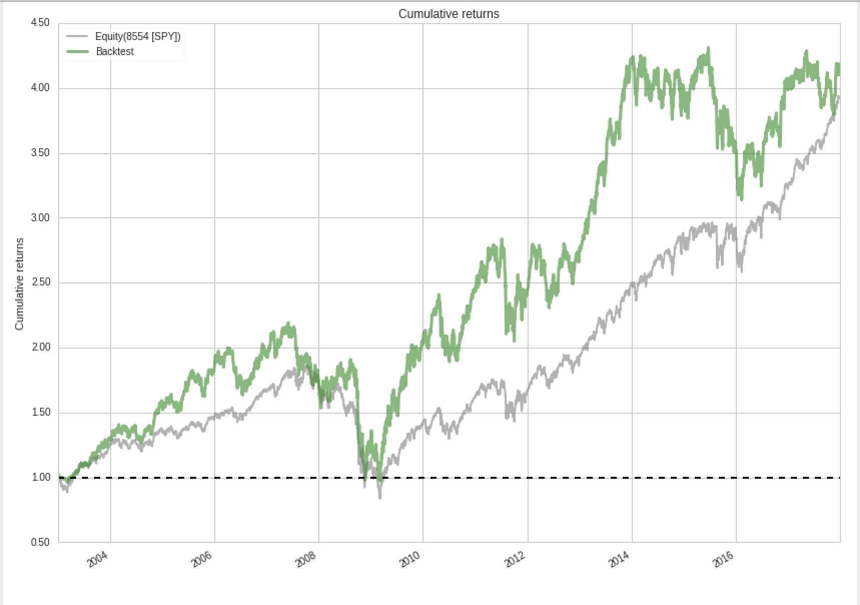
We see a slight positive Sharpe from the output of our backtest, but our cumulative returns in the 15 years studied matches close to that of the S&P 500. Additionally, there was a Max Drawdown of 55.61%, so we do see some significant and prolonged periods of underperformance from this strategy. We do see that, while there were some strong gains post Great Recession, the strategy has had a number of weaker returns relative to the market.
Conclusion
Since Greenblatt's book was first published, value investing has lost some of its luster due to many years of underperformance against the broader market. As Greenblatt himself puts it:
"First, buying good companies at bargain prices makes sense. On average, this is what the magic formula does. Second, it can take Mr. Market several years to recognize a bargain. Therefore, the magic formula strategy requires patience."
It certain seems like it's been more than a couple years. And yet, the Magic Formula lives on as one of the more popular investment strategies. While the theory behind the formula is indeed simple, very small details in how we decide what is considered "good" and "cheap" can make a significant impact to your stock universe. Some of the book's suggestions, like removing stocks with a P/E fo 5 of below, seem to conflict with the stock list generated by Greenblatt's website. That said, our exercise was as much about replicating the book's output as it was about demonstrating a quant workflow, and to that we hope you have found value in this experience.
In the fifth and final installment of this strategy discussion, we'll add some concluding remarks on this strategy, and compare our results to Greenblatt's own performance in running Gotham.