Magic Formula (Part III)

---

---

Backtesting The Magic Formula Using Python in Quantopian and Alphalens

In Part I and Part II of this series, we introduced the Magic Formula made famous by the book The Little Book that Beats the Market, from legendary value investor Joel Greenblatt of Gotham Asset Management LLC. We tried to replicate the screen for the Magic Formula as closely as we could using python through the financial research platform Quantopian. Finally, we compared our list of potential positions compared to that of the official website. In the third part of this strategy discussion, we look to quantify the strength of our screen to determine whether the strategy is a suitable candidate for a full backtest.

Factor Analysis

---

Before we go through with backtesting our signals in Quantopian's IDE (which can be somewhat time consuming), we need a way to make sure that the factors we created have predictive power. Luckily, we can leverage Quantopian's Alphalens tool to easily and efficiently find whether our signals merit further study.

We'll keep the pipeline we created in the previous notebook, but will import a few new modules from alphalens.

from alphalens.performance import mean_information_coefficient
from alphalens.utils import get_clean_factor_and_forward_returns
from alphalens.tears import create_information_tear_sheet, create_returns_tear_sheet, create_full_tear_sheet
                

Now we'll go ahead and create our pipeline from the previous pipeline function that we created in Part II.

factor_data = run_pipeline(make_pipeline(), '2003-1-1', '2018-1-1')
                

For this exercise, we'll run the data from January 1st, 2003 until January 1st, 2018. This covers 15 years of the strategy and should be enough time to give us an idea of whether our factors are worth backtesting. The pipeline will create a ranking based on the Return on Capital and Earning's Yield factors from the Magic Formula. Our hypothesis is that the highest ranked stocks (top 30) will have positive alpha. In order for us to test this hypothesis, we'll need the prices of securities for those 15 years, plus a year out into the future, since we are interested in measuring returns one year out.

pricing_data = get_pricing(factor_data.index.levels[1], '2003-1-1', '2019-1-2', fields='open_price')
                

Now that we have the pricing data, it's pretty much plug and play to create our tearsheet. We'll use the function get_clean_factor_and_forward_returns to get forward returns based on factor bins. The Magic Formula calls for buying the top 30 stocks based on the dual factor ranking, so we should ideally see the highest returns on those higher ranked symbols. The function allows us to set a number of look-forward periods, and while the Magic Formula is designed to have a one year holding period, we'll also look at one month, and six month performance. Finally, we'll break the results out into deciles to get a clear glimpse of the best stocks in the portfolio.

factor_data = get_clean_factor_and_forward_returns(factor = factor_data['sum_rank'],  
                                                   prices = pricing_data,  
                                                   quantiles =10,
                                                   periods = (21,126,252))
                

Now we can create our tearsheet of results

create_full_tear_sheet(factor_data)
                

The results look as we would have hoped.

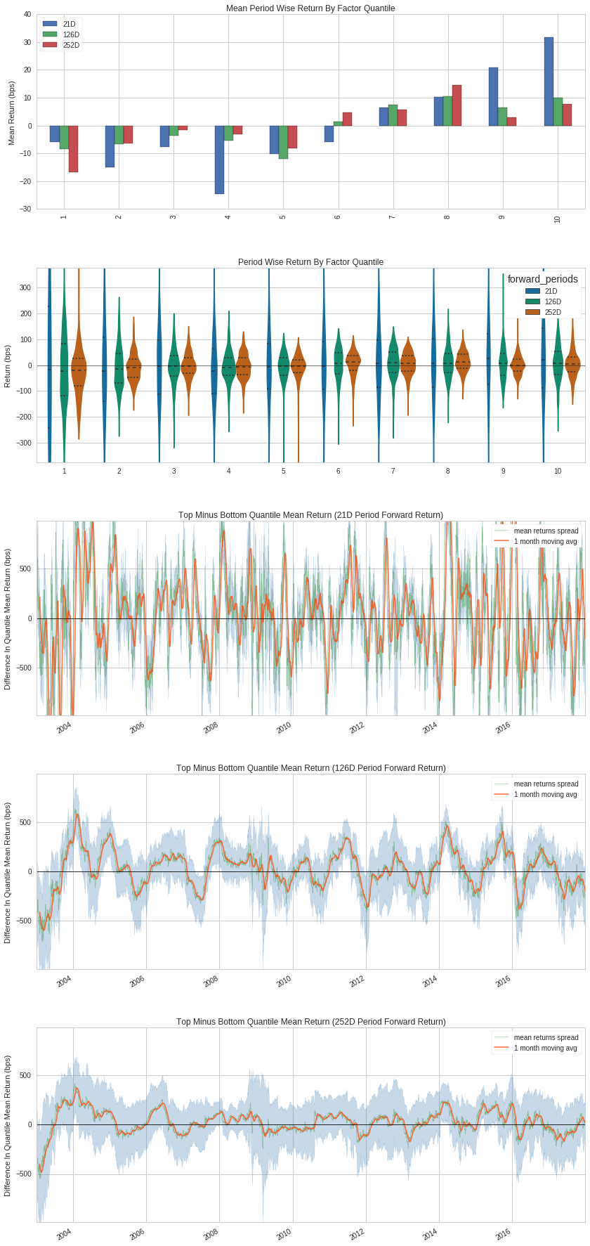
The first bar chart clearly shows that the highest mean return comes from the top decile of ranked factor securities. We also see a general decline in performance as the bins move down in rank. Interestingly, we see our strongest performance from a one month holding period of the top decile of stocks, instead of a one year holding period as defined by the Magic Formula (considerations for taxes are not built into this test model).

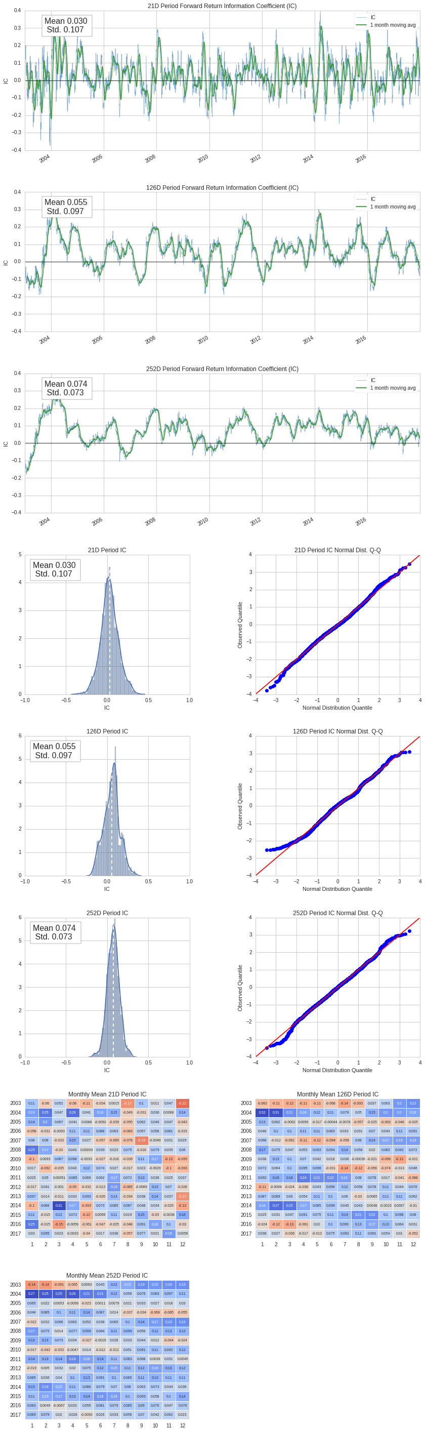
The tearsheet also provides us with the information coefficient (IC). The information coefficient lets us see whether the factor rankings are correlated to future returns. We want to see strong positive mean values for IC. For a one year return (252 Days), we find an Information Coefficient mean of 0.074 with a Standard Deviation of 0.073. We can also study the IC breakdown by month in the heatmap matrix at the bottom.

---

The Takeaway

Based on the positive Information Coefficient and promising decile forward returns breakout, we think that the Magic Formula signal is worthwhile for further study. In the fourth section of this strategy discussion, we will run this pipeline through Quantopian's Algorithm API, to find out how the strategy would have performed over our testing period.