Creating Drop Down Lists In Excel
Drop-Downs Are Useful When Filtering Out Data in Excel. To Do This:
-
Create a Pivot Table to find unique values of the elements you want in your drop down.
Insert > PivotTable -
Group the unique elements into a name that can be referenced
Highlight Cells > Fill in Name Box. -
Go to the cell where you want your drop down, and reference that cell back to the Grouping that has just been created.
Data >
                      Data Validation > Choose Data Type and Source using Grouping name
.
Get the Book: Excel 2019 Bible
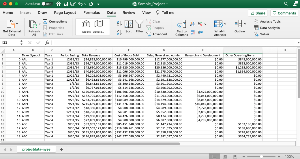
Interacting with spreadsheets can be quite burdensome when the data is large, so it is reasonable to filter out data to only what is needed for study. To that end, Excel can be constructed to have dashboard-like properties, giving an audience a mechanism to select data based on a drop-down menu of items. For this exercise, we walkthrough the precise steps involved in creating a drop-down menu.
Step One: Consolidate Selection
Let's create a drop-down list for the different Ticker Symbols in the sample sheet above. Our first step is to find all the unique instances of these symbols, and while we can do this manually based on a dataset of 20 rows, this can become more challenging as the size of our data increases. There are several ways to do this in Excel, and one simple trick is to create a Pivot Table off the tickers.
We highlight the cells containing the tickers (including the index label), navigate to Insert, and click on
the icon for PivotTable to the left. We accept the default settings to create a table on a new tab, and
navigate to the newly constructed but empty pivot table. We check the box for Ticker Symbol, and make sure that this field is also
under the Rows window. We can now copy and paste these values together somewhere on the spreadsheet.
Step Two: Grouping Symbols
With the unique tickers identified, we can now select these unique symbols and group them together. To accomplish this, we highlight the values of our unique tickers, and replace the name box with a name you want to reference the data to later. In this example, we rename these symbols to the group name of "Tickers".
Step Three: Reference Grouping in a Function
Now that we have a name for the group of symbols we want in our dropdown, we can easily refer back to it using an Excel function. To demonstrate how this work, we'll create another tab in our spreadsheet, and navigate toData, then Data Validation.
A window will open up asking the data type we want to use for our data validation, and in this example we will choose a List. For the
source, we refer back to the group we had just created and named Tickers, press Enter, and voila! A drop-down window has now been
created with the values of the unique symbols from the original data set.